
Introduction
This page proposes some information on Geiger Muller Counters (GMC) with the idea, not to explain the theory of radioactivity (there are many websites that do this very well (and others less ...)) but rather, to help you to build (or choose) a device that, I hope, will be useless to you!
Geiger Muller Counters
A GMC is a measuring device that counts the number of certain particles that pass through its detector.
Our environment produces such particles at more or less significant rates. Below a certain value, we consider that this rate is "normal" and bearable by our body. Beyond another value, the dose is considered to be lethal in a more or less short term. In between, we are in an increasingly dangerous area as the rate increases.
The CGM lets you know which zone you are in.
How a GMC tube works?
One of the main detectors used is the Geiger-Muller tube developed in the 1920s. Its principle is as follows:
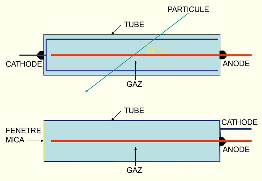
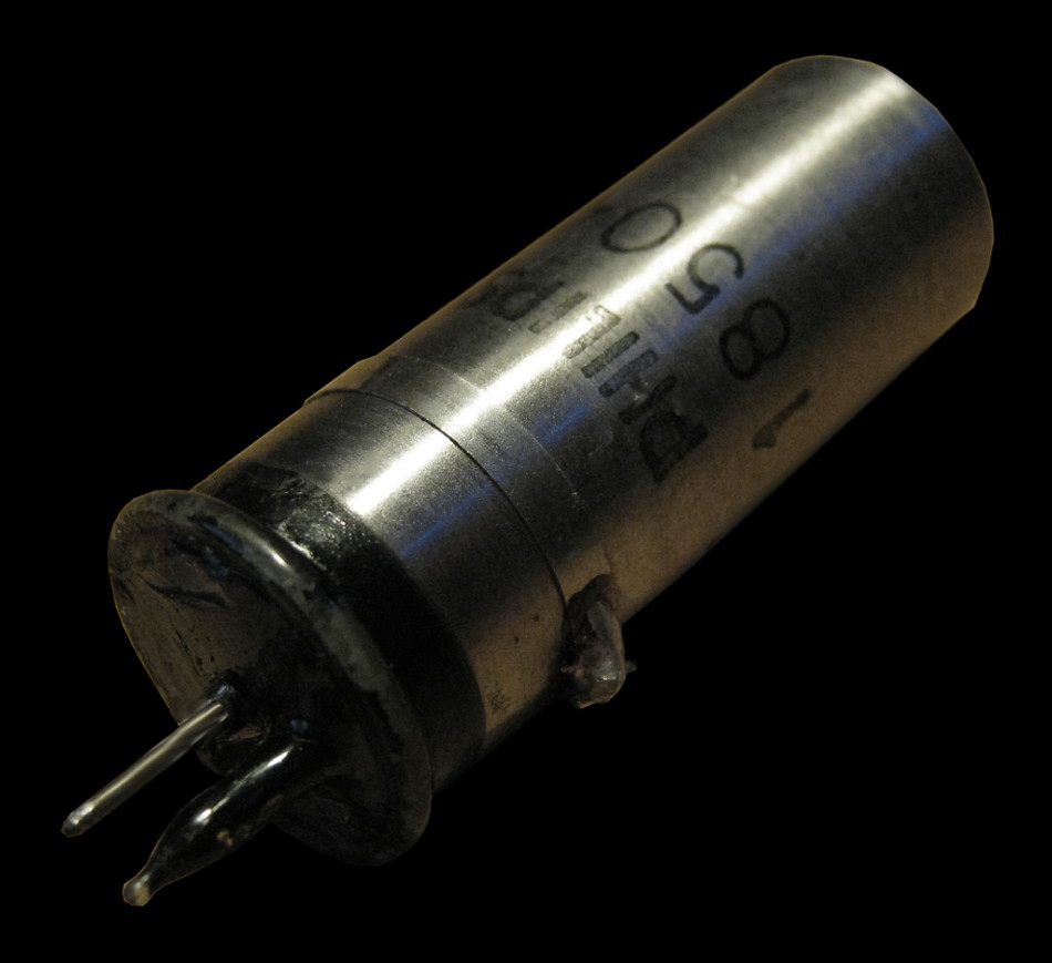
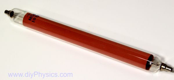
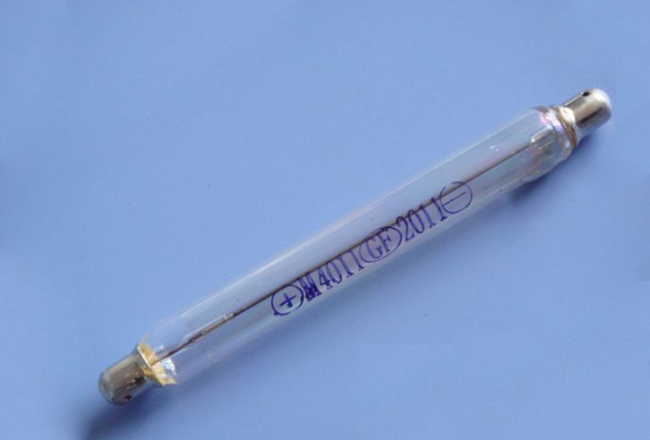
The most classic GM tube has the shape of a cylinder. It is filled with a gas that does not conduct electricity (neon, argon helium, krypton, etc.) under low pressure. Inside this waterproof tube (which is sometimes made of glass) is another metal tube (sometimes it is the body of the tube itself) in which there is an electrode (which is about the length of the tube) which is called cathode. In the center of the cathode is another electrode, a metal rod, which is called an anode. The electrodes are accessible either at each end or grouped on one end of the tube. The SBM20 is a good illustration of this type of tube. The electrodes are accessible at both ends.
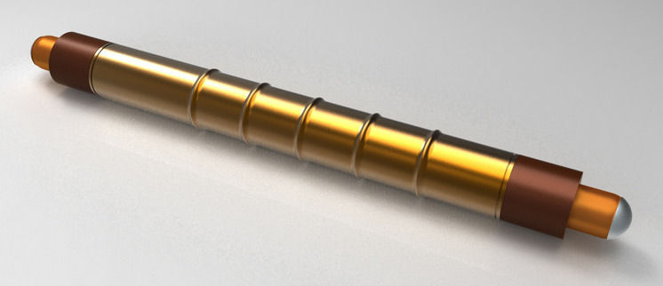
A Russian tube SBM20
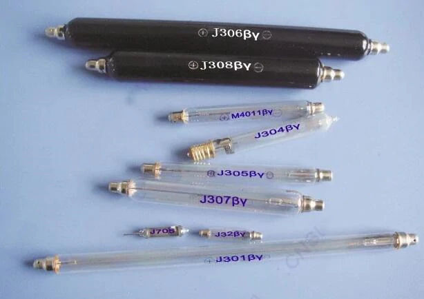
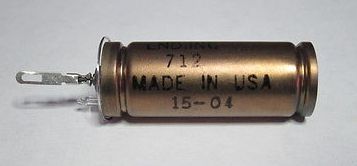
Some tubes are cylinders with a mica window at one end (example, the (LND712). Typically, these tubes are designed to detect Alpha radiation (in addition to Beta and Gamma):
Some tubes have the shape of a disc or a flat box, with a spiral anode, or several anodes in parallel and a large window in mica on one side. These tubes are designed to detect Alpha radiation (in addition to Beta and Gamma). By their shape, they are called "Pancake" tubes.

A Russian pancake tube SI-8B
Let’s go back to our explanation. Between the cathode and the anode, a certain voltage difference is established (in general, several hundred volts). This voltage difference is chosen to be at the limit beyond which the gas could ionize and become conductive.
Under normal conditions, no current flows between the cathode and the anode.
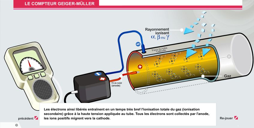
When a particle / radiation crosses the tube, it interacts with the gas and if its energy level is sufficient, it will create negative ions, very mobile electrons and positive ions less mobile than the electrons. These ions are collected by the cathode and the anode which creates a current flow between the two electrodes.
The electrons furthest from the anode will acquire significant kinetic energy during their journey.
This energy is sufficient to ionize other gas molecules near the anode and thereby create a kind of amplification known as the "Townsend discharge".
This ionization will create other positive ions near the anode. Being less mobile, these ions create a positive space charge which will eventually stop the discharge phenomenon.
Little by little, the positive ions will finish their migration towards the cathode. These ions will then regain the electrons they lack which allows them to return to a neutral state. However, this operation will be done by emitting a photon whose energy is sufficient to ionize the gas again, especially since the photon is not stopped by a space charge.
If nothing is done, an avalanche effect can be created and destroy the tube. To avoid this phenomenon, a gas (quenching gas: butane, ethanol, etc.) is introduced, the role of which is to “blow” this effect.
The quenching gas is chosen so that its positive ions do not produce photons when they return to the neutral state. Thus, the positive ions of the main gas will for certain collide with molecules of the quenching gas, pass to the neutral state by transferring their energy to the molecules of the quenching gas which in turn ionize. The positive ions then join the cathode in order to regain electrons but as we mentioned before, without emitting a photon which ends up stopping the avalanche phenomenon.
The animation below comes from the French Atomic Energy Commission (CEA) website (click on the image to see the animation).
During these phenomena, a current flows in the tube which can be detected. Once detected, the role of the GMC is to inform the user of the event. Typically:
- in a sound way, by activating a loudspeaker (the cracklings well known in movies)
- visually via a galvanometer
- visually via a digital display
These three modes are of course not exclusive.
Note that during the conduction time, the tube is no longer able to detect another particle. It has to return to its original state which takes, as we have seen, a certain time. This time, called "dead time", is therefore an important characteristic of a tube since it makes it possible to determine its maximum detection capacity, therefore, for the GMC, the maximum counting rate. In the tubes which are commonly found, the value of the dead time is of the order of 50 to 100 μs.
There is also a "recovery time" or "restitution time" which follows the dead time. This duration is related to the fact that the positive ions take as we have seen a certain time before being captured by the cathode. This electric field decreases the sensitivity of the tube which decreases the counting capacity without canceling it completely. The tube recovers its full characteristics when all the positive ions have been captured by the cathode.
Understanding counting
One difficulty is to understand the rate displayed by the meter. Knowing that 35 particles have been detected in a minute is not very informative if you do not have a reference.
The particle detector (a Geiger-Muller tube in our case) is designed to detect certain particles or radiation. For example, it can be Gamma particles (of the same nature as light, therefore photons), Beta (of the same nature as electrons), Alpha (Helium nucleon composed of two neutrons and two protons).
Some tubes are sensitive to Alpha radiation, others to Beta and Gamma radiation, others still only to Gamma radiation. Tubes detecting Beta and Gamma radiation are the most common.
Ultimately, what matters is what your body can absorb without being too degraded. This is why a unit of measurement, the Sievert, was invented which gives an idea of the biological impact of radiation absorbed by humans.
To convert a number of particles measured into Sievert, a "conversion factor" or "conversion rate" is assigned to each tube according to its sensitivity and the radiation it detects. Unfortunately, this factor is sometimes difficult to determine and obviously does not take into account the fact that certain radiations are or are not detected by a particular tube.
Consequently, the measurement in Sievert given by a GMC is subject to caution.
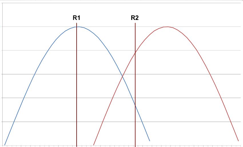
Consider two GM tubes whose sensitivities to different radiations are indicated by the blue and red curves. The abscissa corresponds to the radiations and the ordinate to the sensitivity to these radiations.
Suppose there is a source of radiation R1. The blue tube will detect this radiation, so the count will be greater than 0 while the red tube will detect nothing and will count 0. The conversion to Sievert being the product of this count by a constant conversion factor (say 1 for the need of this example), the GMC using the blue tube will display a certain value in Sievert per unit of time (5) while the GMC using the red tube will display 0.
If we now consider the radiation R2, given the higher sensitivity of the red tube to this radiation, the number of particles counted over a certain period will be larger than for the blue tube, a little more than twice as much. So the Sievert value displayed by the GMC using the red tube will be a little more than twice as large (4) as for the GMC using the blue tube (slightly less than 2).
Obviously, one could decide that the conversion factor of the blue tube must be multiplied by two to obtain the same value in Sievert as the red tube. But in this case, how to consider the value measured for R1 which would also be multiplied by two and which would therefore be worth 10 in this example.
The reason for all this comes from the fact that the tubes do not differentiate the types of radiation that they measure and that the conversion factor is a given constant for a certain type of radiation corresponding to a certain level of energy.
Disappointed? You must not! You just have to know the limits of a GMC and know how to interpret the measurements. In practice, what interests the user will be more the variation of the counting level than its exact value. Knowing that ambient radioactivity has increased by a factor of 10 compared to a measurement in a healthy environment is an interesting indication able to alert you to the dangerousness of the place where you took the measurement.
This is also the reason why, for my part, I prefer to follow the value in counting per minute (CPM) than in Sievert which seems less telling.
Can we differentiate the types of radiation?
Theoretically, no. We just know that we have detected a particle.
However, there is a trick to differentiate with more or less precision the types of radiation. This trick is implemented on the Gamma Scout GMC described below.
Radiation can be stopped by obstacles placed in their path. Thus, Alpha radiation is stopped by a simple thin sheet of aluminum. For Beta radiation, a thicker sheet can also stop them. On the other hand, for gamma radiation, the thickness of the material to be placed to stop them quickly becomes too great for us to consider putting such an obstacle in a portable meter: Some sources give a lead thickness of 6 cm to reduce the radiation intensity by 30%.
Suppose we have a Geiger-Muller tube capable of detecting Alpha, Beta and Gamma radiation.
Take a measurement by putting an obstacle that lets in only the Gamma radiation. Then repeat the measurement by removing the obstacle. Assuming that the radiation source is constant, you will be able to know the Beta and Alpha radiation by difference. The same reasoning applies to distinguish Alpha radiation from Beta and Gamma radiation.
Another possibility is to use several tubes, each detecting only certain types of radiation (for example, Gamma for one tube, Alpha, Beta and Gamma for another) and to proceed by subtracting the measurements via computer processing.
But as already said, these tips have their limits and the CGM is not a good instrument for making an accurate measurement of the various types of radiation.
Normal radioactivity values
The normal radioactivity values measured in CPM vary from tube to tube (and also from place to place). It is generally accepted that values between 0 and 50CPM (typically, 20 to 50CPM for an SBM20) correspond to the ambient radioactivity.
The regulations also set the authorized Sievert values according to the types of population.
Based on the value of 1mSv.year, the maximum hourly value (rate generally displayed on GMC) should be around 0.114µSv.
If your GMC displays 1.14µSv.h, the regulations indicate that populations must be sheltered. From 5.7µSv.h, the population must be evacuated. From 11.4µSv.h, doses of iodines must be dispensed.
Some measurements
Below are some examples of measurements in different environments made by three GMC: :
These measurements were made between June and October 2016. The values in Sievert are orders of magnitude.
| Location | GMC | CPM | mSv/an | Comment |
| Brittany | GammaScout | 18 | 0,4 | Average over 6 months |
| PC-GM5 | 23 | |||
| PC-GM6 | 21 | |||
| Paris | GammaScout | 10 | 0,2 | Radioactivity in Brittany near Rennes is slightly less than twice that in Paris |
| PC-GM5 | 12 | |||
| PC-GM6 | 11 | |||
| Flights Paris-Osaka 07/2016 | GammaScout | 273 | 6,5 | The radioactivity received during a long-haul flight is high. |
| Flights Osaka-Paris 08/2016 | GammaScout | 287 | ||
| Osaka stay 07/2016 | GammaScout | 13 | 0,3 | The average radioactivity is of the same order as that of Paris |
Measuring radiation is sometimes full of surprises. So, one day visiting the Saint-Etienne cathedral in Saint-Brieuc (France, Brittany), I was surprised to find that my meter panicked when I was close to certain floor tiles: those which are very dark. I no longer have the figures in mind (it was around 2000) but I remember that the difference compared to "normal" ambient radioactivity was very significant.
PC-GM5 et PC-GM6 use the same tube. Why count differences? ?
One can imagine slight drifts in manufacturing. Another more likely reason is the difference in design between the two meters. PC-GM6 has a monostable whose adjustment is intended to prevent measurements during the idle time. In practice, I set the monostable to a value greater than the dead time value of the tube. This may explain why PC-GM6 therefore measures slightly fewer pulses than PC-GM5 (sensitivity reduced by around 10%).
Tube models and specifications
Introduction
Except for the Russian tubes from "New Old Stock", it is not easy to find resellers of new tubes or even sometimes, the characteristics of these tubes.
Here are some website addresses of tube manufacturers in 2020. You will see that for some of them, there is no documentation available. For others, it is very incomplete.
- Centronic, UK. No longer very active in 2020.
- Saint Gobain, Crystals, US/France. Seems to no longer produce tubes in 2020.
- LND, manufacturer, US
- Vacutec, Germany
- John Caunt, UK
- Mirion/Canberra, manufacturer, US
- Southern Scientific, reseller, UK.
It should be remembered that certain equipment is subject to the Wassenaar agreements for export authorizations, this perhaps explaining that ...
The DiyGeigerCounter site gives lots of information on all kinds of tubes. I added the references of tubes for which I found some characteristics. The table below provides a summary.
- References are listed alphabetically.
- The sensitivity is given according to 60Co (1st line, Cps at 1 mR/h) and / or 137Cs (2nd line, Cps at 1 mR/h) when available.
- Voltage: in brackets, the recommended voltage.
- Conversion factor: value for converting the number of pulses per minute to microSievert per hour (µSievert.hour = CPM x Conversion factor). When there are several, the first is the one I use. If you have read the previous paragraphs, you know that the value of this factor is questionable.
- When there is a photo, it usually comes from tube sales websites.
- Some data on Chinese tubes is questionable! I put the ones that seemed to me the most credible following overlaps.
Russian detectors
Someone sent me a 2017 directory on Russian radiation detectors (title in English, "Directory of Radiation Receivers and Detectors, 2017, M.L. Baraiochnikov") which can be found here " Справоуник Приемники и детекторы излучений, 2017, М.Л. Бараночников " [Archive] . The number of references is quite staggering (I did not count but it is at least a hundred). In addition, it is better to have some notions of Russian.
Part 2 concerns less this page (although). It relates to "Optical detectors" "Часть вторая оптического излучения" [Archive]
Part 3 is about "photoelectronic optical detectors" "Часть третья фотоэлектронные оптического излучения" [Archive]
There is also an older version of the first document on the net "Приемники и детекторы излучений, 2012, М.Л. Бараночников" [Archive]
Tubes characteristics
 |
 |
 |
 |
 |
 |
 |
 |
|---|---|---|---|---|---|---|---|
| 18503, 18504, 18505, 18506, 18508, 18509, 18510, 18511, 18515, 18516, 18517, 18518, 18520, 18522, 18524, 28525, 18526, 18529, 18533, 18536, 18537, 18538, 18545, 18546, 18548, 18550, 18552, 18553 | the Netherlands (Philips). See catalogue 1965 [archive]. | ||||||

|
α β γ | ? ? |
425-675 (500) |
100µs | 10M | ? | L=43mm, D=15mm. Mica Window. The Netherlands (Philips). Datasheet. |
|
β γ | ? ? |
380-450 (400V) |
? | ? | ? | L=34mm, D=6,5mm. China. Datasheet. |
|
|
β γ | 0,8 ? |
380-480 (400V) |
? | ? | ? | L=205mm, D=10,5mm. China. Datasheet. |
|
|
β γ | 37 ? |
360-440 (380) |
? | ? | ? | L=90mm, D=10,5mm. China. Datasheet. |
|
|
β γ | 44 ? |
380-450 (400V) |
? | 5,1M | 0,00812037 | L=107mm, D=10mm. China. Datasheet. |
|
|
β γ | 50 ? |
360-440 (400V) |
? | ? | ? | L=200mm, D=19mm. China. Datasheet. |
|
|
β γ | ? ? |
380-480 (400V) |
? | ? | ? | L=197mm, D=14mm. China. Datasheet. |
|
|
β γ | 50 ? |
380-480 (400V) |
? | ? | ? | L=143mm, D=18mm. China. Datasheet. |
|
α β γ | 18 ? |
450-650 (500V) |
90µs | 10M | 0.0081208 0,00926 0,00833 0,009 0,01 0,00233 |
L=50mm, D=15mm. US (LND). Mica Window. Used by the Gamma-Scout. Datasheet. |
| LND7317 | α β γ | 58 ? |
475-675 (500V) |
60µs | 4,7M | 0.0024 | L=76,1mm, D=53,6mm. US (LND). Pancake with Mica Window. |
| LND7231 | α β γ | 25 ? |
450-700 (500) |
30µs | 4,7M | ? | D=33mm, h=22mm. US (LND). Pancake with Mica Window. |
| LND7616 | α β γ | 10 ? |
750-950 (760) |
75µs | 1M | ? | L=63,4mm, D=6,4mm. US (LND). Mica Window |
|
γ | ? ? |
780-880 (820) |
? | 8 to 15M | ? | L=260mm, D=21,5mm. Russian. |
|
β γ | ? ? |
360-440 (380V) |
? | ? | 0,00662 | L=90mm, D=10mm. China. Equivalent to SBM20. Datasheet. |
СБМ10
|
β γ | ? ? |
370-480 (400V) |
64µs | ? | ? | L=35mm. Russian. |
|
СБМ20
|
β | 22 | 350-475 (400V) |
190µs | 5,1M | 0.0057 0,00664 0,00504 0,00584 0,00277 |
L=108mm, D=11mm. Russian. |
СБМ21
|
β | ? ? |
370-480 (400V) |
64µs | 3 to 15M | 0,048000 |
|
| SBT9 СБT9 |
α β γ | ? ? |
350-450 (390V) |
100µs | 10M | 0.0117 0.0109 |
L=66mm, D=10mm. Russian. |
СБT10A
|
α β γ | ? ? |
(380) | 50µs | 10M | ? | Mica Window. 10 electrodes, 10M by electrode |
СБT11A
|
α β γ | ? ? |
260-320 (?) |
? | ? | 0.0031 | L=55mm, l=30mm. Russian. |
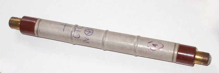
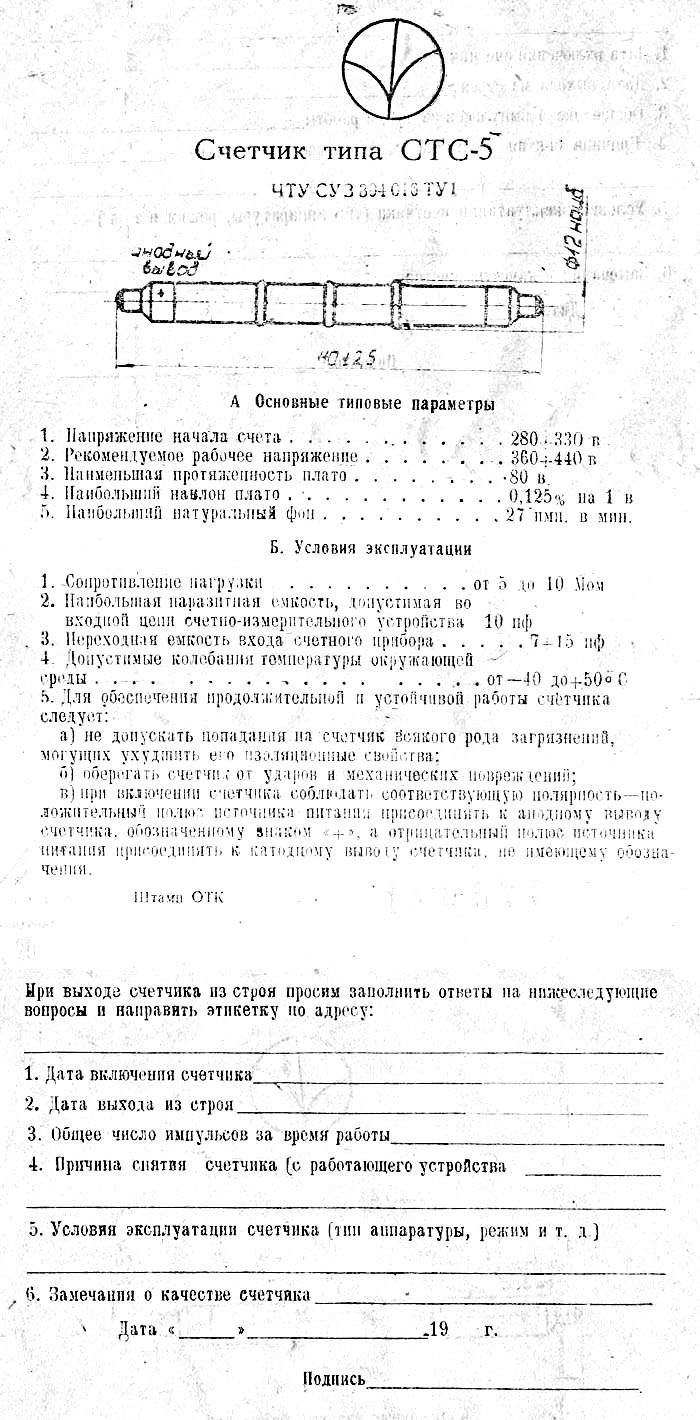
CTC6 |
β γ | ? ? |
390-400 (?) |
? | 5 to 10M | 0.0021 | L=199mm, D=22mm. Russian. |
СИ1Б
|
β | ? ? |
360-440 (?) |
? | 5 to 10M | 0,006000 | Russian. |
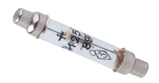
СИ3БГ
|
β γ | ? ? |
380-460 (400) |
? | 10M | 0,044 0,631578 |
L=55mm, D=8mm. Russian. |
СИ8Б
|
β | ? ? |
360-440 (?) |
? | 20M | 0,00232 | D=80mm, L=31,4mm. Russian. Pancake. |
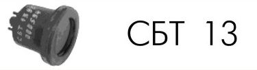
СИ13
|
β | ? ? |
320-450 (?) |
? | ? | ? | D=42mm, L=47mm. Russian. Pancake. 100 - 140 impulsions/s at 1μR/s |
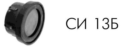
СИ13Б
|
β | ? ? |
350-550 (?) |
? | ? | ? | D=49mm, L=26mm. Russian. Pancake. 350 - 500 impulsions/s at 1μR/s |
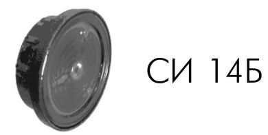
СИ14Б
|
β | ? ? |
350-550 (?) |
? | ? | ? | D=84mm, L=26mm. Russian. Pancake. 300 impulsions/s at 1μR/s |
|
SI16BG СИ16БГ |
β γ | ? ? |
360-440 | ? | >8M | ? | L=110mm, D=12mm. Russian. |
|
SI19G СИ19Г |
γ | ? ? |
360-460 | ? | ? | ? | L=87,4mm, D=10,25mm. Russian. 45 - 61 impulsions/s at 1μR/s |
СИ19БГ-M
|
β γ | ? ? |
360-440 | ? | ? | ? | L=20mm, D=9,3mm. Russian. 1000 - 1500 impulsion/s at 1R/h |
СИ19БГ
|
β γ | ? ? |
350-450 (400) |
? | ? | ? | L=70mm, D=10mm. Russian.Datasheet. |
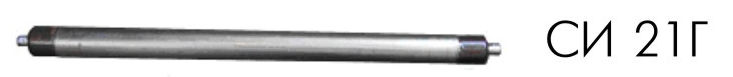
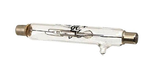
СИ21Г
|
γ | ? ? |
360-480 |
? | ? | ? | L=259,2mm, D=18,25mm. Russian. 285 - 385 impulsion/s at 1μR/s |
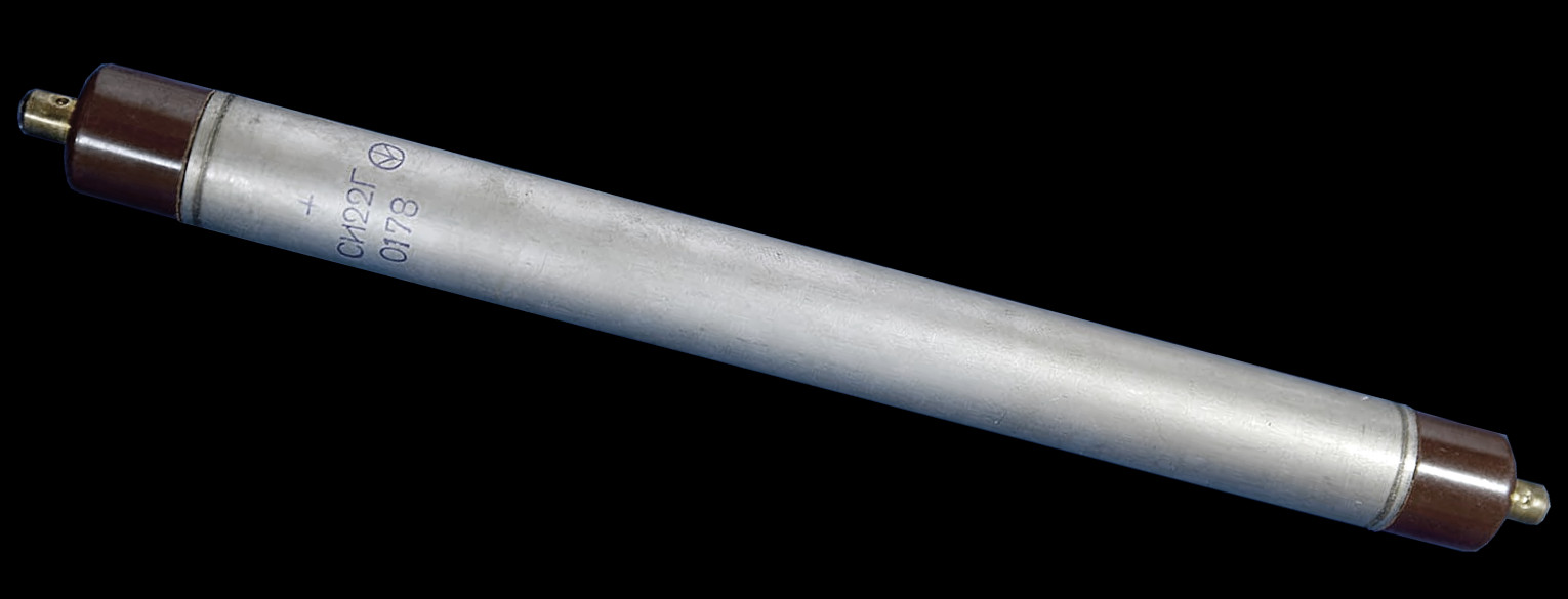
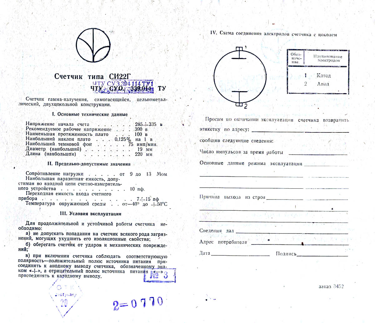
СИ22Г
|
γ | ? ? |
360-440 (400) |
? | 9 to 13M | 0,001714 | L=220mm, D=19mm. Russian. Datasheet. |
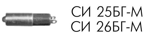
СИ25БГ-М SI26BG-M СИ26БГ-М
|
β γ | ? ? |
360-440 (400) |
? | 9 to 13M | ? | L=42mm, D=10,3mm. Russian. 30 impulsions/s at 4μR/s. |
СИ25Г
|
γ | ? ? |
382-398 (?) |
? | 1,5M | ? | L=55mm, D=10mm. Russian. Pas cher. 0,2 - 0,35μA/R/h |
| SI29BG СИ29БГ |
β γ | ? ? |
360-440 (400V) |
95µs | ? | 0.0082 0.01 |
L=61,5mm, D=10mm. Russian. |
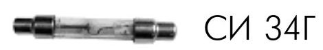
СИ34Г
|
γ | ? ? |
360-440 |
? | ? | ? | L=55mm, D=8mm. Russian. 30 - 70 impulsion/s at 1R/h |
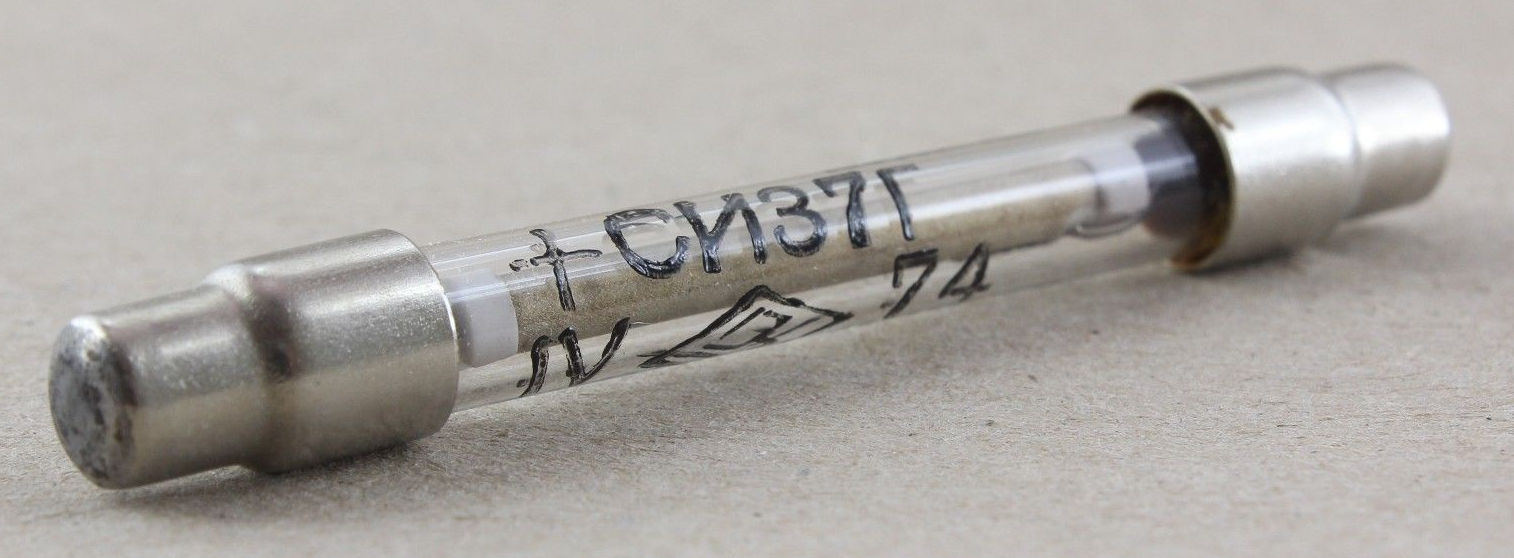
СИ37Г
|
γ | ? ? |
350-550 (390) |
? | ? | ? | L=56mm, D=8mm. Russian. 1900 - 2700 impulsion/s at 1R/h |

СИ38Г
|
γ | ? ? |
500-600 (550) |
? | 2,1M | ? | L=55mm, D=10mm. Russian. 8,8 - 13,2 impulsions/s at 1R/h |
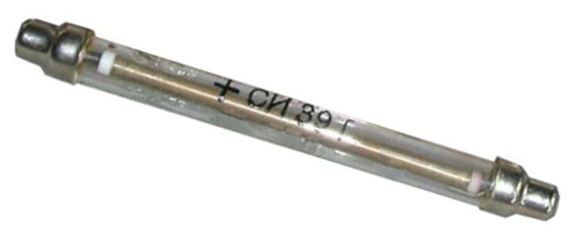
|
SI39BG СИ39БГ |
? ? |
380-460 (?) |
? | ? | ? | L=55mm, D=10mm. Russian. 188-282 impulsion/s at 1R/h | |
СИ39Г
|
γ | ? ? |
360-440 (395) |
? | >2,2M | ? | L=93,5mm, D=15mm. Russian. 19,5 - 21,5 impulsions/s at 1μR/s. |
CTC5
|
β | ? ? |
360-440 | ? | 5 to 10M | ? | L=110mm, D=12mm. Russian. Replaced by SBM20 Datasheet. |
| S800 1188 | β γ | ? ? |
850-1000 (925) |
? | ? | ? | L=51,3mm, D=18,4mm. US/FR (St Gobain). Datasheet. |
| S800 1192 | β γ | ? 65 |
850-1000 (900) |
20µS | 3,3M | ? | L=12,7mm, D=44,5mm. US/FR (St Gobain). Pancake. Datasheet. |
| S800 1193 | β γ | ? 65 |
475-675 (500) |
40µS | 3,3M | ? | L=12,7mm, D=44,5mm. US/FR (St Gobain). Pancake. Datasheet. |
| S800 1210 and 1209 | β γ | ? ? |
850-1050 (950) |
? | ? | ? | L=110mm, D=15,4mm. US/FR (St Gobain). Datasheet. |
| S800 1211, 1212 and 1240 | β γ | ? ? |
850-1050 (950) |
? | ? | ? | L=123,4mm, D=18,5mm. US/FR (St Gobain). Datasheet. |
| S800 1213 and 1214 | β γ | ? ? |
650-800 (725) |
? | ? | ? | L=124,2mm, D=15,4mm. US/FR (St Gobain). Datasheet. |
| S800 1215 and 1216 | β γ | ? ? |
650-800 (725) |
? | ? | ? | L=175,8mm, D=15,4mm. US/FR (St Gobain). Datasheet. |
| S800 1217 and 1218 | β γ | ? ? |
850-1050 (950) |
? | ? | ? | L=224,5mm, D=15,4mm. US/FR (St Gobain). Datasheet. |
| S800 1219 and 1220 | β γ | ? ? |
650-800 (725) |
? | ? | ? | L=71,1mm, D=15,4mm. US/FR (St Gobain). Datasheet. |
| S800 1222 | α β γ | ? ? |
450-650 (550) |
? | ? | ? | L=34mm, D=14,5mm. US/FR (St Gobain). Datasheet. |
| S800 1224 | γ | ? ? |
450-600 (525) |
? | ? | ? | L=34mm, D=14,5mm. US/FR (St Gobain). Datasheet. |
| S800 1225 | γ | ? ? |
500-750 (625) |
? | ? | ? | L=201,4mm, D=15,4mm. US/FR (St Gobain). Datasheet. |
| S800 1227 | γ | ? ? |
450-650 (500) |
? | ? | ? | L=193mm, D=18,4mm. US/FR (St Gobain). Datasheet. |
| S800 1229 | β γ | ? ? |
850-1000 (925) |
? | ? | ? | L=220,8mm, D=15,4mm. US/FR (St Gobain). Datasheet. |
| S800 1230 and 1232 | β γ | ? ? |
850-1050 (950) |
? | ? | ? | L=221,3mm, D=15,4mm. US/FR (St Gobain). Datasheet. |
| S800 1235 | α β γ | ? ? |
450-650 (550) |
? | ? | ? | L=34mm, D=14,5mm. US/FR (St Gobain). Mica Window. Datasheet. |
| S800 1236 and 1237 | α β γ | ? ? |
850-950 (900) |
? | ? | ? | L=62,5mm, D=28,6mm. US/FR (St Gobain). Mica Window. Datasheet. |
| S800 1241 | β γ | ? ? |
650-800 (725) |
? | ? | ? | L=62,2mm, D=15,4mm. US/FR (St Gobain). Datasheet. |
| S800 1245 | γ | ? ? |
500-650 (575) |
? | ? | ? | L=29,2mm, D=7,8mm. US/FR (St Gobain). Datasheet. |
| S800 1254 | β γ | ? ? |
400-500 (450) |
? | ? | ? | L=135,9mm, D=18,5mm. US/FR (St Gobain). Datasheet. |
| S800 1255 | β γ | ? ? |
400-500 (450) |
? | ? | ? | L=222,3mm, D=18,5mm. US/FR (St Gobain). Datasheet. |
| S800 1262 | β γ | ? | 850-1050 (950) |
? | ? | ? | L=115,8mm, D=15,4mm. US/FR (St Gobain). Datasheet. |
| T2000/500 | α β γ | ? 58 |
450-600 (500) |
50µs | 3,3M | ? | L=53,6mm, D=15,3mm. US (Canberra). Pancake, Mica Window 44,5mm.Datasheet. |
| T2000/900 | α β γ | ? 58 |
850-1000 (900) |
50µs | 3,3M | ? | L=53,6mm, D=15,3mm. US (Canberra). Pancake, Mica Window 44,5mm. Datasheet. |
| T2006/500 | α β γ | ? 58 |
450-600 (500) |
50µs | 3,3M | ? | L=53,6mm, D=31,7mm. US (Canberra). Pancake, Mica Window 44,5mm. Datasheet. |
| T2006/900 | α β γ | ? 58 |
850-1000 (900) |
50µs | 3,3M | ? | L=53,6mm, D=31,7mm. US (Canberra). Pancake, Mica Window 44,5mm. Datasheet. |
| T2011/500 | α β γ | ? 25 |
450-600 (500) |
40µs | 3,3M | ? | L=32,5mm, D=33,5mm. US (Canberra). Pancake, Mica Window 27,9mm. Datasheet. |
| T2011/900 | α β γ | ? 25 |
850-1000 (900) |
40µs | 3,3M | ? | L=32,5mm, D=33,5mm. US (Canberra). Pancake, Mica Window 27,9mm. Datasheet. |
| VA-Z-115.1 | β γ | ? ? |
(450) | ? | 2M | 0,0044 | L=53mm, D=14mm. Allemand. Ne pas confondre avec VA-Z-114NR pas sensible du tout. |
| ZP1000 ZP1001 |
? ? |
1600-2400 | ? | 10M | ? | Thermal neutron. The Netherlands (Philips). See catalogue 1965 [archive]. | |
| ZP1010 | ? ? |
900-1900 | ? | 10M | ? | Thermal neutron. The Netherlands (Philips). See catalogue 1965 [archive]. | |
| ZP1020 | ? ? |
2300-3800 | ? | 10M | ? | Thermal neutron. The Netherlands (Philips). See catalogue 1965 [archive]. | |
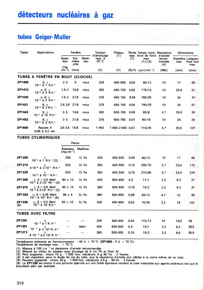
| ZP1200 | γ | ? ? |
400-600 | 90/12µs | 10M | ? | L=56mm, D=17mm. France (RTC/Philips). Datasheet. |
| ZP1201 | γ | ? ? |
400-600 | 110/12µs | 10M | ? | L=58mm, D=19,5mm. France/The Netherlands (RTC/Philips). Datasheet. |
| ZP1301 | γ | ? ? |
500-600 | 13/1µs | 2,2M | ? | L=28,5mm, D=6,2mm. France/The Netherlands (RTC/Philips). Datasheet. |
| ZP1313 | γ | ? ? |
500-650 | 15/2µs | 2,2M | ? | L=36,9mm, D=8,9mm. France/The Netherlands (RTC/Philips). Datasheet. |
| ZP1210 | γ | ? ? |
400-500 | 200/70µs | 2,7M | ? | L=170mm, D=23,4mm. France/The Netherlands (RTC/Philips). Datasheet. |
| ZP1220 | γ | ? ? |
400-500 | 210/90µs | 2,7M | ? | L=270mm, D=23,4mm. France/The Netherlands (RTC/Philips). Datasheet. |
| ZP1300 | β γ | ? ? |
500-600 | 11/1µs | 2,2M | ? | L=27mm, D=6,2mm. France/The Netherlands (RTC/Philips). Datasheet. |
| ZP1310 | β γ | ? ? |
500-650 | 15/2µs | 2,2M | ? | L=37mm, D=6,2mm. France/The Netherlands (RTC/Philips). Datasheet. |
| ZP1322 | β γ | ? ? |
500-650 | 15/2µs | 4,7M | ? | L=55mm, D=10mm. France/The Netherlands (RTC/Philips). Datasheet. |
| ZP1330 | β γ | ? ? |
450-800 | 110/25µs | 2,2M | ? | L=142mm, D=19mm. France/The Netherlands (RTC/Philips). Datasheet 1, Datasheet 2. |
| ZP1400 | β γ | ? ? |
450-600 | 90/12µs | 10M | ? | L=55mm, D=17mm. France/The Netherlands (RTC/Philips). Mica Window 9mm. Datasheet. |
| ZP1410 | α β γ | ? ? |
450-700 | 175/15µs | 10M | ? | L=57mm, D=25,9mm. France/The Netherlands (RTC/Philips). Mica Window 19,8mm. Datasheet. |
| ZP1430 | α β γ | ? ? |
450-700 | 190/25µs | 10M | ? | L=57mm, D=34mm. France/The Netherlands (RTC/Philips). Mica Window 27,8mm. Datasheet. |
| ZP1431 | β γ | ? ? |
450-700 | 190/25µs | 10M | ? | L=57mm, D=34mm. France/The Netherlands (RTC/Philips). Mica Window 27,8mm. Datasheet. |
| ZP1442 | β γ | ? ? |
500-700 | 65/8µs | 4,7M | ? | L=30mm, D=25,9mm. France/The Netherlands (RTC/Philips). Mica Window 19,8mm. Datasheet. |
| ZP1450 | α β γ | ? ? |
850-1000 (900) |
40µs | 3,3M | ? | L=32,5mm, D=33,5mm. UK (Centronic). Pancake, Mica Window 27,9mm. |
| ZP1452 | β γ | ? ? |
500-750 | 65/18µs | 10M | ? | L=34mm, D=34mm. France/The Netherlands (RTC/Philips). Mica Window 27,8mm. Datasheet. |
| ZP1600 | X | ? ? |
1600-2000 (1450) |
110/25µs | 10M | ? | L=127mm, D=25,9mm. France/The Netherlands (RTC/Philips). Mica Window 19,8mm. Datasheet. |
COMMERCIAL GMC
In 2019, the CGM consumer offer is quite significant when you consider the devices supplied on the shelf and the kits.
All modern devices are microprocessor-based, which makes it possible to count and calculate averages, or even to memorize counts over a more or less long period. The display is on a liquid crystal display or OLED, which can be purely alphanumeric or graphic.
Besides the functional aspects, what distinguishes the GMC are the tubes used. Some are very efficient, others less. One merits that we focus on in particular:
The Gamma Scout
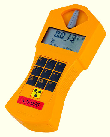
The GMC Gamma Scout is probably the most efficient GMC on the consumer market in 2019.
- The GMC uses an efficient tube, the LND712 which can detect Alpha, Beta and Gamma radiation.
- Its autonomy in permanent operation is ten years with a simple lithium battery.
- It can store the measurements over different periods (minutes, hours, day, etc.).
- It is possible to download the measurements to process them on a computer.
- The display is permanent and allows you to choose between several units including the microSievert per hour. It also has a bargraph for analog measurement of radioactivity.
- Finally, it filters the types of radiation (Alpha + Beta + Gamma or Beta + Gamma or Gama only).
If the hardware is well designed, the software aspects are more disappointing. In particular, the communication protocol between the GMC and the host has obviously been designed by neophytes... We can also regret the absence of some functionalities, including counting in CPM.
The others GMC
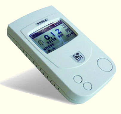
Many modern meters, like the RADEX 1503+, the MKC-03CA, the kits, use a Russian tube SBM20 which detects Gamma and Beta radiation. This tube has a good reputation and it is also the one I used for some of my achievements.
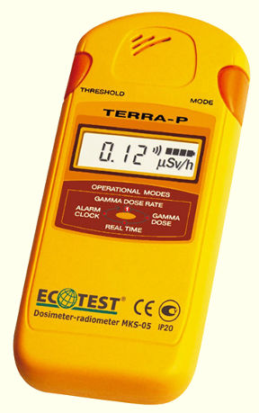
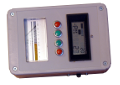
GMC Ecotest Terra-P and Radex 1503
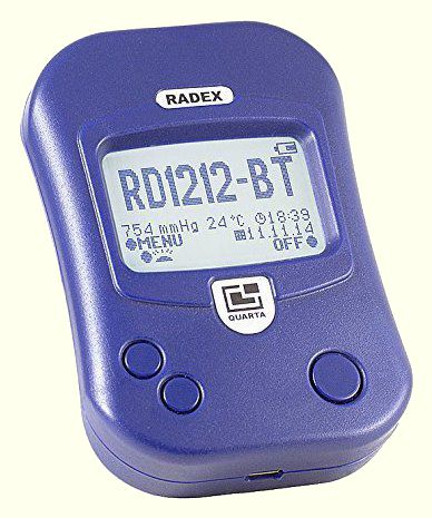
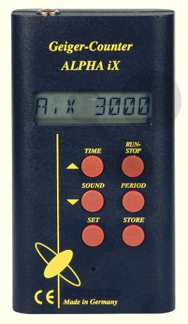
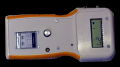
GMC Radex 1212 and Alpha iX
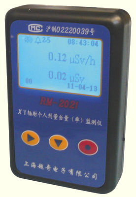
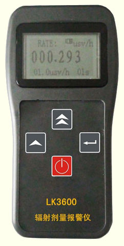
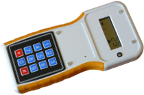
Chinese GMC rm2012 and lk3600
On the other aspects, they are far below the performance of the Gamma-Scout, in particular in terms of power consumption. Most have only an autonomy of a few hundred hours (typically 400 to 500 hours), even those which are described as low consumption. The cause: an archaic conception, knowing that the Gamma-Scout with its 10 years of autonomy has been available since the end of the 1990s. Because of their poor conception, I would tend to advise you against them. Admittedly, they are often less expensive than a Gamma-Scout (in 2015, around 300 € for the standard model which is quite sufficient against 150 € for a Radex RD1503+) but in use they will be disappointing.
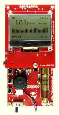
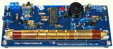
MyGeiger and Arduino Base Kit Meters
In terms of power consumption, the kits are not better designed than most commercial meters, but they allow you to experiment.
However, it is possible to experiment while having a very low power consumption meter like the PC-GM3 to 8 (up to 10 years of autonomy in my version) whose schematics and software I propose on this site. By their performance, they are very close to Gamma-Scout, less expensive and you can improve their functionality by modifying the proposed software.
Tips for making a CGM
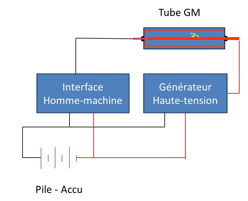
The block diagram of a CGM is very simple :
- A source of energy (battery).
- A low-voltage to high-voltage converter (400V to 1000V depending on the tubes).
- A user interface (loudspeaker, galvanometer, digital counter, graphic display).
Since the 1990s, the user interface has most often been a digital display, for example, with liquid crystal, controlled by a microprocessor, coupled to a sound system (crackling sounds when a particle is detected).
The voltage converter is the most delicate element because it is often the most energy-consuming. It is not uncommon to find assemblies consuming several mA, or even ten mA. For my part, I use a ready-made assembly, the imex 38-56. Its power consumption is of the order of a few µA to a few tens of µA. In addition, it operates from 3V which is compatible with the supply of microprocessors.
For the tube, the choice depends on what you want to detect. An SBM20 makes it possible to have a master key for a modest cost but which does not detect alpha radiation.
For the user interface, it is possible to simply carry out a processing by microprocessor whose consumption is of the order of 10 μA, including display (see my realisations below) after).
High voltage adjustment
To adjust the high-voltage (if it is adjustable), a standard multimeter is not sufficient because its impedance is generally too low (typically, 10Mohms for an electronic multimeter, 20 to 40kohms per volt for an analog multimeter) currents involved: the high-voltage generator is not designed to supply large currents and the voltage will collapse during the measurements.
It is necessary to build a measurement probe with a resistance of the order of 1Gohms. The generator voltage is calculated as follows:
Vactual is the generator voltage. Vread is the voltage read from the multimeter. Rprobe is the resistance of the probe (1Gohms). Rmultimeter is the input impedance of the multimeter (in general, 10Mohms).
Tube connection
The anode of the tube is connected to the high-voltage supply via a resistor which limits the current when the avalanche phenomenon occurs following the detection of a particle. The value of this resistance is given by the manufacturer of the tube.
All the authors agree on one point, the resistor must be connected as close as possible to the tube. If the tube is connected by an electric wire to the resistance, the length of this wire must be very short: maximum 2 to 3 cm if possible.
For measurement, this can be done at the anode or at the cathode.
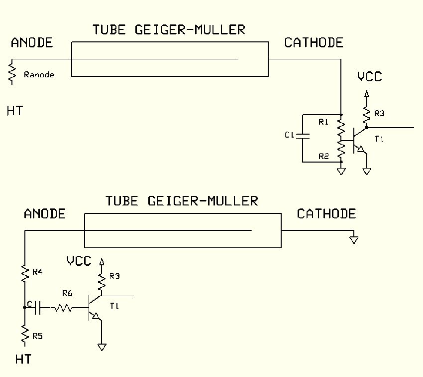
Connection at the cathode level is the simplest, but some authors advise against it. With this arrangement, the cathode is floating relative to the mass. It seems that this floating mass can disturb the extinction of the avalanche phenomenon and cause parasitic voltage peaks which distort the measurement.
The measurement at the anode, with cathode to ground, seems to be more reliable. This connection is recommended by certain authors and by certain manufacturers (see for example the specifications of LND tubes).
For my part, PC-GM3 and PC-GM4 use the measurement on the cathode and they seem to work properly except that... from time to time, I have parasitic oscillations with certain tubes. The PC-GM5 model is a simplified version of the PC-GM3 and PC -GM4 and use the measurement on the anode.
My GMCs
Over time, I have built or acquired several Geiger Muller counters. This chapter shows these realizations and proposes variants which could help those who want to get started in the realization of such devices.
For details, the GMC are generally describe on the measures page (in French). The software that comes with certain GMC is in the resources section.
PC-GM1
When I built my first GMC in the 1980s, I didn't give it a special name. But since I made others, I decided to name these GMCs PC-GMx. PC, I'll let you guess, GM for Geiger-Muller and x, the model number.
PC-GM1 is in fact the realization of a schematic from the Elektor magazine in April 1980 .
It is completely conventional and the article gives all the indications concerning its conception and its realization. It has a counting output (TTL pulse) allowing it to be connected to a computer or a laboratory GMC. Its main drawback? Its size probably but above all, its power consumption.
I deconstructed it in the late 1990s to recover certain components. So I have no photo to propose.
PC-GM2
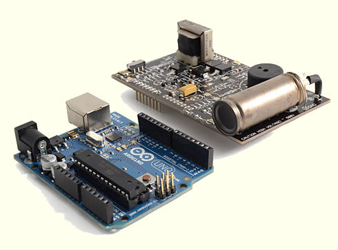
 I built this GMC when my Gamma Scout , bought in 2000/2001, decided to stop working in 2012 more battery wear (11 years of battery life anyway!). And by changing it (which is not planned), I had to do something wrong because I put it down permanently (probably, the high-voltage generator). Rather than repairing it, I preferred to build another one by recovering the tube ( LND712 ) from the Gamma Scout. This allowed me to get my hands on Arduino. The result is PC-GM2. My added value on this model was limited to the design of the meter software and to a PC software, GeigerPC which allows you to control the GMC when it is connected and to record measurements.
The disadvantage of this GMC is its high power consumption (of the order of 40mA). The fault comes from the design of the Arduino-Unos and the high-voltage circuit board. A notable improvement would be to replace the high-voltage generator with the one I used on my other meters. But do not dream, the Arduino Uno is not an experimentation board for low power consumption. Therefore, it is better to look at the following GMCs.
PC-GM3
My goal was to build a GMC consuming less than 100µA, including permanent display. Mission accomplished thanks to the use of a trick that I did not see elsewhere at the time when I designed it. It consists of using an RTC (Real Time Clock ) circuit as an event counter and letting the processor rest most of the time. Average consumption is around 20µA.
Of course I abandoned the Arduino for a module based on the Texas Instrument MSP430f449 processor. As for the high voltage generator, it is a Imex-38-56 module whose power consumption is compatible with the objective.
I released the GMC software for free download. And as for PC-GM2, it is connectable to the software GeigerPC which allows to control the meter when it is connected and to record measurements.
The trick in question is interesting when the processor does not have a counter operating in low power consumption mode. The Texas processor used has such a counter. This considerably simplifies assembly. The PC-GM5 model is therefore a simplified version of the PC-GM3 and PC-GM4 which directly uses the processor counter.
PC-GM4
 PC-GM4 was originally the prototype for PC-GM3.
Once PC-GM3 finished, I cleaned up the prototype which became PC-GM4.
PC-GM4 was originally the prototype for PC-GM3.
Once PC-GM3 finished, I cleaned up the prototype which became PC-GM4.
What are the changes?
- There is no buzzer to report "tics".
- There is a meter to display instant particle detection.
For the rest (logic part, tube, program ...), PC-GM4 is identical to PC-GM3.
I released the counter software for free download. And as for PC-GM2/3, it is connectable to the software GeigerPC which allows to control the meter when it is connected and to make recordings of measures.
PC-GM5
 PC-GM5 is a simplified version of PC-GM3 .
It directly uses a processor counter to count instead of the PCF8583. This is possible with the processor used because the counter remains active in low consumption mode. Furthermore, the measurement is made at the anode and no longer at the cathode.
PC-GM5 is a simplified version of PC-GM3 .
It directly uses a processor counter to count instead of the PCF8583. This is possible with the processor used because the counter remains active in low consumption mode. Furthermore, the measurement is made at the anode and no longer at the cathode.
Due to certain design choices, consumption is slightly higher than that of PC-GM3 and is around 30µA.
I released the GMC software for free download. And as for PC-GM2/3/4, it is connectable to the software GeigerPC which allows to control the meter when it is connected and to do measurement records.
PC-GM6
 PC-GM6is a simplified version of PC-GM4.
As PC-GM5, it directly uses a processor counter to count at instead of PCF8583. This is possible with the processor used because the counter remains active in low power consumption mode. Furthermore, the measurement is made at the anode and no longer at the cathode.
PC-GM6is a simplified version of PC-GM4.
As PC-GM5, it directly uses a processor counter to count at instead of PCF8583. This is possible with the processor used because the counter remains active in low power consumption mode. Furthermore, the measurement is made at the anode and no longer at the cathode.
But the main improvement is the use of a double monostable CD4098. One is used to generate a clean signal on the processor counter, in eliminating any transient oscillations. The signal length can be adjusted to be greater than or equal to the dead time of the tube used.
the other is used to activate the galvanometer. The duration of the pulse is adjustable to allow it to be adapted to the characteristics of the galvanometer used.
The average power consumption measured using a digital oscilloscope is around 25~30µA (no alarm, galvanometer disabled). Variation consumption is more sensitive to particle detection than for other models due to the use of monostables. They consume very little at rest but generate a "fairly high" current peak when a pulse is taken into account.
I released the GMC software for free download. And as for PC-GM2/3/4/5, it can be connected to the software GeigerPC which allows to control the meter when it is connected and to do measurement records.
PC-GM7
The GM tube is a survival from the past. Fragile, expensive, delicate in its implementation, requiring a high voltage supply, there is no doubt that in the short term, it is doomed to be replaced by semiconductor detectors.
In practice, several realizations of amateurs based on PIN diode are proposed on the net. For cost reasons, the BPW34 diode is the most used (€1 in 2015).
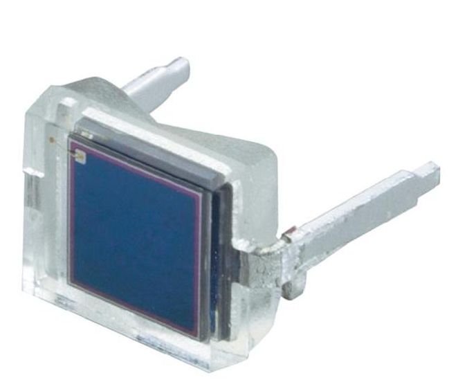
bpw34 diode
The picture is misleading. The diode is really very small! The sensitive surface is around 7mm². The dimension of the diode itself is of the order of 5mm by 5mm.
You will find below some links on realizations based on this diode or others. Most of them use operational amplifiers for the analog part, resulting in a fairly high consumption, generally varying between 1ma and 10mA. The result is quite mixed: the meters are less sensitive and consume more than a traditional Geiger-Muller tube assembly (around 30µA for my work, including microncontroller). Only one assembly claims very low consumption (2µA).
- A radiation Sensor Shield (broken link).
- Clectronic, A radiation sensor.
- Elektor, radiation meter.
- Alan's Lab, Photodiode Gamma Ray Detector.
- Jameco, kit instruction.
- Bricolsec, détecteur de radioactivité.
- Burkhard Kainka, Measure Gamma Rays with a Photodiode.
- Opengeiger.de
- www.teviso.com
- RH electronic
- CircuitSalad
- California university and Berkeley National Laboratory.
- Build and Test of A Gamma Radiation.
While waiting to find a complete realization on this site, here are some particularities which emerge from these numerous articles:
- The sensitivity does not seem very good. We can improve it by putting diodes in parallel but in this case, we also increases the parasitic capacity of the assembly which decreases the signal intensity. In the end, it seems that beyond two diodes, the gain in sensitivity is marginal, even negative.
One solution is to put several diode-preamplification sets in parallel in order to avoid this inconvenience. It is not the price of a few transistors and resistors of this preamplification which will significantly change the price of the set. - The diode (and its preamplification) must be encapsulated in a metal case which isolates it from light and ambient noise.
- Some precribe the use of operational amplifiers for signal amplification. The reason given is that the amplifiers operational benefit from long years of design and are more efficient than a transistor assembly. Great gain, possibility of effective filtering to eliminate noise below 20kHz are strong arguments for the use of these components.
For the moment, PC-GM7 is only in the planning stage. For the IT part, the idea is to reuse what has already been implemented for the PC-GM3 to PC-GM6 GMC.
PC-GM8
 PC-GM8 uses an MSP430FR4133. For the analog part, I designed a PCB. The schematic end the PCB accepts SBM20, J305 or an LND712 (but other tubes can also be used).
The main change is the use of a multiplexer which allows the processor to control the analog alarms (buzzer and LED). It also has an e-paper display for displaying information that varies little. Its consumption is a little higher than my other meters based on MSP430.
PC-GM9
 PC-GM9 uses an MSP430FR6989. For the analog part, I designed a PCB. It accepts for an SBM20, J305 or an LND712 (but other tubes can also be used).
PC-GM9 is an evolution and above all a simplification of PC-GM8. It no longer has an e-paper display but has a keyboard which is more useful than the rotary switch. Its greater storage capacity provides a history of approximately 8000 measurements (i.e. one year of measurement at the rate of one measurement per hour).
WATCHES AND RADIOACTIVITY
The old luminescent watches used radium to make the indications of the dial and the hands visible at night. This process was abandoned in the 1960s. You will find many articles on this subject on the net.
If, like me, you practice watchmaking as an amateur and you sometimes buy lots of mechanical watches for a few euros, you can come across old radioactive watches. For my part, in 2018, out of twelve watches bought in a batch, 6 were radiocative. And not just a little ...
Where I live, in Brittany, the ambient radioactivity is around 20 to 22 CPM with an SBM20 tube (see my work). A simple watch hand raises the GMC to 750 CPM (or, approximately, 37msV / year), 24 times more than normal in Brittany and almost 40 times more than normal in Paris, which is starting to do a lot .
If in doubt, disassemble the hands and the dial and store everything in a metal box in a place away from people and specify the danger on the box.
